[Dacon] 음성 분류 경진대회

---

데이콘의 “음성 분류 경진대회”에 참여하여 작성한 글이며, 음성 데이터에 대한 데이터 증강(Data Augmentation)과 음성 특성 추출(Feature Extraction) 구현 방법을 서술합니다.

코드실행은 Google Colab의 CPU, Standard RAM 환경에서 진행했습니다.

➔ 데이콘에서 읽기

     

0. Import Packages

• 주요 라이브러리 불러오기

import numpy as np
import pandas as pd
import random as rn
import os

from scipy.io import wavfile
import librosa

import matplotlib.pyplot as plt
import seaborn as sns
import IPython.display as ipd
import librosa.display

import warnings
warnings.filterwarnings("ignore")
%matplotlib inline

     

1. Load and explore dataset

• 데이터 불러오기

train = pd.read_csv('/content/drive/MyDrive/Speech_classification/train.csv')
test = pd.read_csv('/content/drive/MyDrive/Speech_classification/test.csv')

     

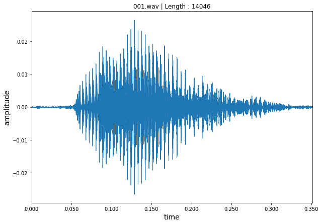
• 한 음성의 Waveplot을 확인해보겠습니다.

a_filename = '/content/drive/MyDrive/Speech_classification/dataset/train/001.wav'
samples, sample_rate = librosa.load(a_filename)

plt.figure(figsize=(10, 7))

# plt.plot(np.linspace(0, sample_rate/len(samples), len(samples)), samples)
librosa.display.waveplot(samples, sr=40000)

plt.xlabel('time', fontsize = 14)
plt.ylabel('amplitude', fontsize = 14)
plt.title('001.wav | Length : ' + str(len(samples)))

plt.show()

     

print(sample_rate)
print(samples)

    22050
    [0.00013066 0.00016804 0.00014106 ... 0.00017342 0.00017514 0.        ]

     

• 한 음성 샘플에 대한 Spectrogram을 생성하겠습니다.
  ↪ Short term Fourier transform (STFT)의 Magnitude를 DB-스케일로 변환하여 Spectrogram을 생성합니다.

samples, sample_rate = librosa.load(a_filename)
X = librosa.stft(samples)  # data -> short term FT
Xdb = librosa.amplitude_to_db(abs(X))

plt.figure(figsize=(12, 3))
plt.title('001.wav spectrogram | Length : ' + str(len(samples)))
librosa.display.specshow(Xdb, sr = sample_rate, x_axis='time', y_axis='hz')   
plt.colorbar()
plt.show()

     

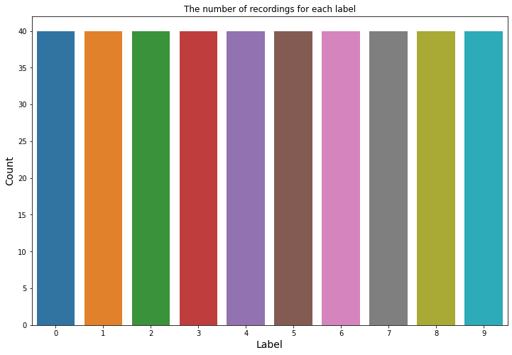
• train.csv에는 train 폴더에 위치한 음성 파일들의 이름과 라벨 컬럼이 포함되어 있습니다. label 컬럼은 0과 9사이의 정수로 구성됩니다.

train.head()

      file_name  label
    0   001.wav      9
    1   002.wav      0
    2   004.wav      1
    3   005.wav      8
    4   006.wav      0

print(train['label'].unique())

    [9 0 1 8 7 4 5 2 6 3]

     

• 데이터가 클래스 균형을 이루고 있습니다.

plt.figure(figsize=(12, 8))
sns.countplot(train['label'])

plt.title("The number of recordings for each label")
plt.ylabel("Count", fontsize = 14)
plt.xlabel("Label", fontsize = 14)
plt.show()

file_name = train['file_name']
train_path = '/content/drive/MyDrive/Speech_classification/dataset/train/'

     

• 데이터들의 길이가 모두 다릅니다.

all_shape = []
for f in file_name:
  data, sample_rate = librosa.load(train_path + f, sr = 20000)
  all_shape.append(data.shape)

print(all_shape[:5])
print("Max :", np.max(all_shape, axis = 0))
print("Min :", np.min(all_shape, axis = 0))

    [(12740,), (13126,), (12910,), (9753,), (17572,)]
    Max : [19466]
    Min : [7139]

     

2. Data Augmentation

• 모델의 일반화 능력 향상을 위해, 기존의 음성데이터에 Perturbation을 추가하여 새 음성데이터를 생성합니다.

↪ Noise 추가, Time Stretching, Pitch 변환

# noise 추가
def noise(sample):
    noise_amp = 0.01*np.random.uniform()*np.amax(sample)
    sample = sample + noise_amp*np.random.normal(size = sample.shape[0])
    return sample

# time stretching
def stretch(sample, rate = 0.8):
    stretch_sample = librosa.effects.time_stretch(sample, rate)
    return stretch_sample

# pitch 변환
def pitch(sample, sampling_rate, pitch_factor = 0.8):
    pitch_sample = librosa.effects.pitch_shift(sample, sampling_rate, pitch_factor)
    return pitch_sample

     

3. Feature Extraction

• 모델링에 사용할 만한 몇가지 Feature Extraction 방법을 소개하겠습니다.

(1) ZCR ^{Zero Crossing Rate}

↪ 특정 프레임에서 신호의 부호(Sign)가 변경되는 빈도입니다. (i.e., 신호의 부호 변화율)

(2) Chroma Shift

↪ 파형(Waveform) 또는 Power Spectrogram으로 생성한 크로마그램(Chromagram) 입니다.

(3) Mel spectrum

↪ 오디오 신호(Time Domain)에 Fast Fourier Transform(FFT)를 적용하여 얻은 주파수 영역(Frequency Domain)의 스펙트럼(Spectrum) 입니다.

↪ Mel Filter Bank를 사용한 필터링 과정을 거쳐 Mel 스펙트럼을 생성합니다.

(4) MFCC ^{Mel-Frequency Cepstral Coefficient}

↪ Mel 스펙트럼에서 Cepstral 분석을 통해 고유한 음향 특성을 추출한 지표입니다.

(5) RMS ^{Root Mean Square}

↪ 오디오 평균 음량을 측정하는 데 사용되는 값입니다.

def extract_features(sample):
    # ZCR
    result = np.array([])
    zcr = np.mean(librosa.feature.zero_crossing_rate(y = sample).T, axis=0)
    result=np.hstack((result, zcr)) 

    # Chroma_stft
    stft = np.abs(librosa.stft(sample))
    chroma_stft = np.mean(librosa.feature.chroma_stft(S = stft, sr = sample_rate).T, axis=0)
    result = np.hstack((result, chroma_stft))

    # MelSpectogram
    mel = np.mean(librosa.feature.melspectrogram(y = sample, sr = sample_rate).T, axis=0)
    result = np.hstack((result, mel)) 

    # MFCC
    mfcc = np.mean(librosa.feature.mfcc(y = sample, sr = sample_rate).T, axis=0)
    result = np.hstack((result, mfcc)) 

    # Root Mean Square Value
    rms = np.mean(librosa.feature.rms(y = sample).T, axis=0)
    result = np.hstack((result, rms)) 

    return result

     

• Noise 추가, Time Stretching, Pitching 방법들을 통해 한 음성데이터 샘플 당 (1, 162) 크기의 Feature를 (3, 162) 로 증강(Augmentation) 합니다.

def get_features(path):

    sample, sample_rate = librosa.load(path)
    
    # without augmentation
    res1 = extract_features(sample)
    result = np.array(res1)
    
    # sample with noise
    noise_sample = noise(sample)
    res2 = extract_features(noise_sample)
    result = np.vstack((result, res2)) 
    
    # sample with stretching and pitching
    str_sample = stretch(sample)
    sample_stretch_pitch = pitch(str_sample, sample_rate)
    res3 = extract_features(sample_stretch_pitch)
    result = np.vstack((result, res3)) 
    
    return result

     

labels = train['label']
x, y = [], []
for f, label in zip(file_name, labels):
    feature = get_features(train_path + f)
    for fe in feature:
        x.append(fe)
        y.append(label)

X = np.array(x)
Y = np.array(y)

print("Shape of X:", np.shape(X))
print("Shape of Y:", np.shape(Y))

    Shape of X: (1200, 162)
    Shape of Y: (1200,)

     

---

Reference

1. Speech Emotion Recognition by SHIVAM BURNWAL