소비자 데이터 기반 소비 예측하기 | 데이콘
💸 소비자 데이터를 분석하고 Elasticnet, LightGBM, XGBoost와 같은 머신러닝 회귀 모델을 활용하여 소비를 예측하는 방법을 소개합니다.
KEYWORDS
소비 예측 딥러닝, 소비 예측 머신러닝, 소비 예측 파이썬, Forecasting Income, Elasticnet, LightGBM, XGBoost
데이콘의 “소비자 데이터 기반 소비 예측 경진대회”에 참여하여 작성한 글이며, 코드실행은 Google Colab의 CPU, Standard RAM 환경에서 진행했습니다.
➔ 데이콘에서 읽기
0. Import Packages
1
2
3
4
5
6
7
8
9
10
11
12
13
14
15
16
17
18
19
20
21
22
23
24
25
26
27
28
29
30
31
32
33
!pip install folium==0.2.1
!pip install markupsafe==2.0.1
!pip install -U pandas-profiling

import numpy as np
import pandas as pd
import matplotlib
import matplotlib.pyplot as plt
import sklearn
import pandas_profiling
import seaborn as sns
import random as rn
import os
import scipy.stats as stats
import datetime
import calendar

from sklearn.preprocessing import PowerTransformer
from sklearn.preprocessing import LabelEncoder
from sklearn.model_selection import train_test_split

from sklearn.model_selection import GridSearchCV, cross_val_score, RepeatedKFold
from sklearn import metrics

from sklearn.linear_model import ElasticNet
from xgboost import XGBRegressor
from lightgbm import LGBMRegressor

from collections import Counter
import warnings

%matplotlib inline
warnings.filterwarnings(action='ignore')
- 주요 라이브러리 버전 확인
1
2
3
4
5
6
print("numpy version: {}". format(np.__version__))
print("pandas version: {}". format(pd.__version__))
print("matplotlib version: {}". format(matplotlib.__version__))
print("scikit-learn version: {}". format(sklearn.__version__))
print("xgboost version: {}". format(xgb.__version__))
print("lightgbm version: {}". format(lgb.__version__))
    numpy version: 1.21.6
    pandas version: 1.3.5
    matplotlib version: 3.2.2
    scikit-learn version: 1.0.2
    xgboost version: 0.90
    lightgbm version: 2.2.3
1. Load and Check Dataset
- 데이터 불러오기
1
2
3
4
5
train = pd.read_csv('/content/drive/MyDrive/Consumer_spending_forecast/dataset/train.csv')
test = pd.read_csv('/content/drive/MyDrive/Consumer_spending_forecast/dataset/test.csv')

print(train.shape)
train.head()
(1108, 22)
       id  Year_Birth   Education Marital_Status   Income  Kidhome  Teenhome  \
    0   0        1974      Master       Together  46014.0        1         1
    1   1        1962  Graduation         Single  76624.0        0         1
    2   2        1951  Graduation        Married  75903.0        0         1
    3   3        1974       Basic        Married  18393.0        1         0
    4   4        1946         PhD       Together  64014.0        2         1

      Dt_Customer  Recency  NumDealsPurchases  ...  NumStorePurchases  \
    0  21-01-2013       21                 10  ...                  8
    1  24-05-2014       68                  1  ...                  7
    2  08-04-2013       50                  2  ...                  9
    3  29-03-2014        2                  2  ...                  3
    4  10-06-2014       56                  7  ...                  5

       NumWebVisitsMonth  AcceptedCmp3  AcceptedCmp4  AcceptedCmp5  AcceptedCmp1  \
    0                  7             0             0             0             0
    1                  1             1             0             0             0
    2                  3             0             0             0             0
    3                  8             0             0             0             0
    4                  7             0             0             0             1

       AcceptedCmp2  Complain  Response  target
    0             0         0         0     541
    1             0         0         0     899
    2             0         0         0     901
    3             0         0         0      50
    4             0         0         0     444

    [5 rows x 22 columns]
- Pandas Profiling Report 생성하기
1
2
3
pr = train.profile_report()
pr.to_file('/content/drive/MyDrive/Consumer_spending_forecast/pr_report.html')
pr
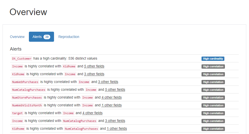
Summary of Pandas profiling : Alert
High Correlation
Income-Kidhome-NumWebPurchases-NumStorePurchases-NumStorePurchases-NumWebVisitsMonth-AcceptedCmp1-AcceptedCmp5-targetNumDealsPurchases-Teenhome
High Cardinality
Dt_customer고객이 회사에 등록한 날짜를 의미하기 때문에 중복도가 낮은 데이터입니다.
- Cardinality가 높다 <-> 중복되는 값이 적다
2. EDA | Exploratory Data Analysis
id: 샘플 아이디,Year_Birth: 고객 생년월일,Education: 고객 학력Marital_status: 고객 결혼 상태,Income: 고객 연간 가구 소득Kidhome: 고객 가구의 자녀 수,Teenhome: 고객 가구의 청소년 수,Dt_Customer: 고객이 회사에 등록한 날짜Recency: 고객의 마지막 구매 이후 일수,NumDealsPurchases: 할인된 구매 횟수,NumWebPurchases: 회사 웹사이트를 통한 구매 건수NumCatalogPurchases: 카탈로그를 사용한 구매 수,NumStorePuchases: 매장에서 직접 구매한 횟수NumWebVisitsMonth: 지난 달 회사 웹사이트 방문 횟수AcceptedCmp(1-5): 고객이 (1-5) 번째 캠페인에서 제안을 수락한 경우 1, 그렇지 않은 경우 0Complain: 고객이 지난 2년 동안 불만을 제기한 경우 1, 그렇지 않은 경우 0Response: 고객이 마지막 캠페인에서 제안을 수락한 경우 1, 그렇지 않은 경우 0target: 고객의 제품 총 소비량
Data Type
- Numeric (10) :
id,Year_Birth,Income,Recency,NumDealsPurchases,NumWebPurchases,NumCatalogPurchases,NumStorePurchases,NumWebVisitsMonth,target - Categorical (12) :
Education,Marital_Status,Kidhome,Teenhome,Dt_Customer,AcceptedCmp(1~5),Complain,Response
- 결측치가 없습니다.
1
train.isnull().sum()
    id                     0
    Year_Birth             0
    Education              0
    Marital_Status         0
    Income                 0
    Kidhome                0
    Teenhome               0
    Dt_Customer            0
    Recency                0
    NumDealsPurchases      0
    NumWebPurchases        0
    NumCatalogPurchases    0
    NumStorePurchases      0
    NumWebVisitsMonth      0
    AcceptedCmp3           0
    AcceptedCmp4           0
    AcceptedCmp5           0
    AcceptedCmp1           0
    AcceptedCmp2           0
    Complain               0
    Response               0
    target                 0
    dtype: int64
1
test.isnull().sum()
    id                     0
    Year_Birth             0
    Education              0
    Marital_Status         0
    Income                 0
    Kidhome                0
    Teenhome               0
    Dt_Customer            0
    Recency                0
    NumDealsPurchases      0
    NumWebPurchases        0
    NumCatalogPurchases    0
    NumStorePurchases      0
    NumWebVisitsMonth      0
    AcceptedCmp3           0
    AcceptedCmp4           0
    AcceptedCmp5           0
    AcceptedCmp1           0
    AcceptedCmp2           0
    Complain               0
    Response               0
    dtype: int64
1
2
df_train = train.copy()
df_test = test.copy()
(1) Outliers
id와target을 제외한 수치적(Numerical) 데이터의 이상치(Outlier) 들을 IQR 기법을 활용하여 찾아줍니다.
1
2
3
4
5
6
7
8
9
10
11
12
13
14
numeric_fts = ['Year_Birth', 'Income', 'Recency', 'NumDealsPurchases', 'NumWebPurchases', 'NumCatalogPurchases', 'NumStorePurchases', 'NumWebVisitsMonth']

train_outlier_ind = []
for i in numeric_fts:
  Q1 = np.percentile(df_train[i],25)
  Q3 = np.percentile(df_train[i],75)
  IQR = Q3-Q1
  train_outlier_list = df_train[(df_train[i] < Q1 - IQR * 1.5) | (df_train[i] > Q3 + IQR * 1.5)].index
  train_outlier_ind.extend(train_outlier_list)

train_outlier_ind = Counter(train_outlier_ind)
train_multi_outliers = list(k for k,j in train_outlier_ind.items() if j > 2)

print("The number of train outliers :", len(train_multi_outliers))
The number of train outliers : 0
- Train 데이터에는 IQR 기법으로 탐지되는 이상치가 없는 사실이 확인됩니다.
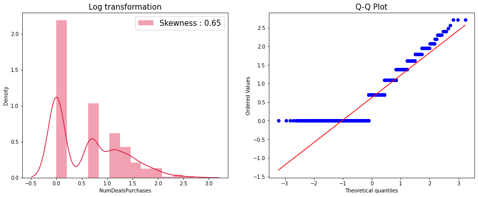
(2) Transformation
- 왜곡된 분포는 모델 학습에 안좋은 영향을 줄 수 있습니다. 높은 왜도(Skewness)를 가지고 있는
NumDealsPurchases변수에 대하여 몇가지 변환함수를 적용하겠습니다.
1
print(df_train[numeric_fts].skew())
    Year_Birth            -0.439100
    Income                 0.291634
    Recency               -0.061310
    NumDealsPurchases      2.264245
    NumWebPurchases        1.289607
    NumCatalogPurchases    1.099499
    NumStorePurchases      0.653689
    NumWebVisitsMonth      0.299000
    dtype: float64
1
2
3
4
5
6
7
8
9
10
fig = plt.figure(figsize = (16,6))
ax1 = fig.add_subplot(1,2,1)
ax2 = fig.add_subplot(1,2,2)

sns.distplot(df_train['NumDealsPurchases'], ax = ax1, label='Skewness : {:.2f}'.format(df_train['NumDealsPurchases'].skew()))
ax1.legend(loc='best', fontsize = 15)

stats.probplot(df_train['NumDealsPurchases'], plot = ax2)
plt.title("Q-Q Plot", fontsize = 15)
plt.show()

Log transformation
1
2
3
4
5
6
7
8
9
10
11
12
13
log_trans = df_train['NumDealsPurchases'].map(lambda i: np.log(i) if i > 0 else 0)

fig = plt.figure(figsize = (16,6))
ax1 = fig.add_subplot(1,2,1)
ax2 = fig.add_subplot(1,2,2)

sns.distplot(log_trans, ax = ax1, color='crimson', label='Skewness : {:.2f}'.format(log_trans.skew()))
ax1.legend(loc='best', fontsize = 15)
ax1.set_title('Log transformation', fontsize = 15)

stats.probplot(log_trans, plot = ax2)
ax2.set_title("Q-Q Plot", fontsize = 15)
plt.show()
Yeo-Johnson transformation
1
2
3
4
5
6
7
8
9
10
11
12
13
14
15
16
jy = PowerTransformer(method = 'yeo-johnson')
jy.fit(df_train['NumDealsPurchases'].values.reshape(-1, 1))
x_yj = jy.transform(df_train['NumDealsPurchases'].values.reshape(-1, 1))

fig = plt.figure(figsize = (16,6))
ax1 = fig.add_subplot(1,2,1)
ax2 = fig.add_subplot(1,2,2)

sns.distplot(x_yj, ax = ax1, color='crimson', label='Skewness : {:.5f}'.format(np.float(stats.skew(x_yj))))
ax1.legend(loc='best', fontsize = 15)
ax1.set_title('Yeo-Johnson transformation', fontsize = 15)

stats.probplot(x_yj.reshape(x_yj.shape[0]), plot = ax2)
ax2.legend(['Lambda : {:.2f}'.format(np.float(jy.lambdas_))], loc='best', fontsize = 15)
ax2.set_title("Q-Q Plot", fontsize = 15)
plt.show()

- 조금 더 정규 분포 직선과 비슷해진 사실을 Q-Q Plot을 통해 확인 가능합니다.
- 데이터 전처리에는 Yeo-Johnson Transformation을 사용했습니다.
1
2
df_train['NumDealsPurchases'] = x_yj
df_train['NumDealsPurchases'].head()
    0    2.258975
    1   -0.801066
    2    0.146388
    3    0.146388
    4    1.846930
    Name: NumDealsPurchases, dtype: float64
1
2
3
4
test_jy = PowerTransformer(method = 'yeo-johnson')
test_jy.fit(df_test['NumDealsPurchases'].values.reshape(-1, 1))
test_x_yj = test_jy.transform(df_test['NumDealsPurchases'].values.reshape(-1, 1))
df_test['NumDealsPurchases'] = test_x_yj
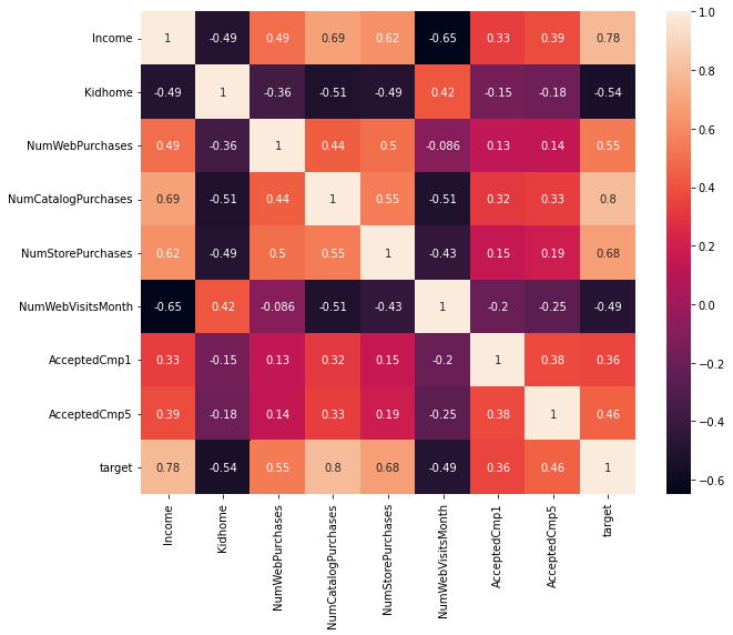
(3) Correlation
- 앞서 수행한 Pandas Profiling Report의 Alert 섹션을 참고하여 상관계수를 계산했습니다.
1
2
3
4
5
6
7
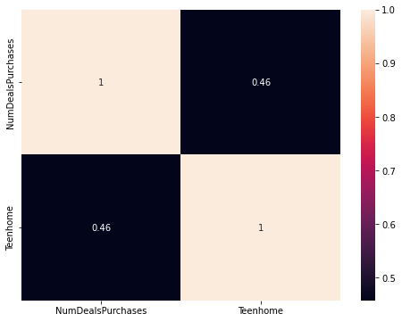
corr_fts1 = ['Income', 'Kidhome', 'NumWebPurchases', 'NumCatalogPurchases', 'NumStorePurchases', 'NumWebVisitsMonth', 'AcceptedCmp1', 'AcceptedCmp5', 'target']
corr_fts2 = ['NumDealsPurchases', 'Teenhome']
plt.figure(figsize = (10,8))
sns.heatmap(df_train[corr_fts1].corr(), annot=True)
plt.show()
1
2
3
4
plt.figure(figsize = (8,6))
sns.heatmap(df_train[corr_fts2].corr(), annot=True)

plt.show()
독립 변수 간의 높은 상관 관계는 다중 공선성을 유발합니다.
해당 문제는 변수 선택, 차원 축소, 규제 등의 방법으로 해결할 수 있고, 필자는 모델에 규제를 주는 역할을 하면서 다중 공선성의 영향을 적게 받는다고 알려진 결정 트리(Decision Tree) 기반의 모델을 사용하겠습니다.
1
2
train_dataset = df_train.copy()
test_dataset = df_test.copy()
3. Feature Engineering
(1) Dt_Customer 변수 : 날짜 데이터 다루기
Dt_Customer변수는 회사 등록일을 뜻 합니다. 회사에 등록된 시점에 대한 정보를 유지하면서 모델링에 사용할 수 있는 새 수치형 변수를 생성하겠습니다.
↪ 가장 과거 시점의 회사 등록일로부터 며칠이 지났는지를 뜻하는 Pass_Customer 변수를 새롭게 생성합니다.
1
train_dataset["Dt_Customer"]
    0       21-01-2013
    1       24-05-2014
    2       08-04-2013
    3       29-03-2014
    4       10-06-2014
               ...
    1103    31-03-2013
    1104    21-10-2013
    1105    16-12-2013
    1106    30-05-2013
    1107    29-10-2012
    Name: Dt_Customer, Length: 1108, dtype: object
1
2
3
4
train_dataset["Dt_Customer"] = pd.to_datetime(train_dataset["Dt_Customer"], format='%d-%m-%Y')
test_dataset["Dt_Customer"] = pd.to_datetime(test_dataset["Dt_Customer"], format='%d-%m-%Y')

train_dataset["Dt_Customer"]
    0      2013-01-21
    1      2014-05-24
    2      2013-04-08
    3      2014-03-29
    4      2014-06-10
              ...
    1103   2013-03-31
    1104   2013-10-21
    1105   2013-12-16
    1106   2013-05-30
    1107   2012-10-29
    Name: Dt_Customer, Length: 1108, dtype: datetime64[ns]
1
2
print(f'Minimum date: {train_dataset["Dt_Customer"].min()}')
print(f'Maximum date: {train_dataset["Dt_Customer"].max()}')
    Minimum date: 2012-07-31 00:00:00
    Maximum date: 2014-06-29 00:00:00
1
2
3
4
5
6
7
train_diff_date = train_dataset["Dt_Customer"] - train_dataset["Dt_Customer"].min()
test_diff_date = test_dataset["Dt_Customer"] - test_dataset["Dt_Customer"].min()

train_dataset["Pass_Customer"] = [i.days for i in train_diff_date]
test_dataset["Pass_Customer"] = [i.days for i in test_diff_date]

train_dataset["Pass_Customer"].head()
    0    174
    1    662
    2    251
    3    606
    4    679
    Name: Pass_Customer, dtype: int64
(2) Year_Birth to Age
Year_Birth변수를 활용하여 고객의 나이를 뜻하는Age변수를 새롭게 생성했습니다.한국나이로 계산했습니다.
1
2
print("Minimum birth :", train_dataset["Year_Birth"].min(), "\nMaximum birth :", train_dataset["Year_Birth"].max(), "\n")
train_dataset["Year_Birth"].head()
    Minimum birth : 1893
    Maximum birth : 1996
    0    1974
    1    1962
    2    1951
    3    1974
    4    1946
    Name: Year_Birth, dtype: int64
1
2
3
4
train_dataset["Age"] = 2022 - train_dataset["Year_Birth"] + 1
test_dataset["Age"] = 2022 - test_dataset["Year_Birth"] + 1

train_dataset["Age"].head()
    0    49
    1    61
    2    72
    3    49
    4    77
    Name: Age, dtype: int64
(3) AcceptedCmp(1~5) 와 Response 변수로 새 Feature 생성
위 여섯개의 변수는 고객이 1~5 번째와 마지막 캠페인에서 제안을 수락한 경우 1, 아닌 경우 0 값을 가집니다.
이 변수들을 활용하여 캠페인에서 제안을 수락한 횟수를 나타내는
AcceptCount변수를 새롭게 생성하겠습니다.
1
2
3
4
train_dataset["AcceptCount"] = train_dataset["AcceptedCmp1"] + train_dataset["AcceptedCmp2"] + train_dataset["AcceptedCmp3"] + train_dataset["AcceptedCmp4"] + train_dataset["AcceptedCmp5"] + train_dataset["Response"]
test_dataset["AcceptCount"] = test_dataset["AcceptedCmp1"] + test_dataset["AcceptedCmp2"] + test_dataset["AcceptedCmp3"] + test_dataset["AcceptedCmp4"] + test_dataset["AcceptedCmp5"] + test_dataset["Response"]

train_dataset["AcceptCount"].head()
    0    0
    1    1
    2    0
    3    0
    4    1
    Name: AcceptCount, dtype: int64
1
print("Minimum count :", train_dataset["AcceptCount"].min(), "\nMaximum count :", train_dataset["AcceptCount"].max(), "\n")
    Minimum count : 0
    Maximum count : 5
Train 데이터에서 캠페인 제안을 여섯번 모두 수락한 경우는 없습니다.
기존 변수와
target과의 상관 관계를 확인하겠습니다.
1
train_dataset[['Year_Birth', 'AcceptedCmp1','AcceptedCmp2','AcceptedCmp3','AcceptedCmp4','AcceptedCmp5', 'Response','target']].corr()
                    Year_Birth  AcceptedCmp1  AcceptedCmp2  AcceptedCmp3  \
      Year_Birth      1.000000     -0.050053     -0.034204      0.066802
      AcceptedCmp1   -0.050053      1.000000      0.198530      0.052213
      AcceptedCmp2   -0.034204      0.198530      1.000000      0.052513
      AcceptedCmp3    0.066802      0.052213      0.052513      1.000000
      AcceptedCmp4   -0.111485      0.184717      0.328941     -0.083690
      AcceptedCmp5   -0.010873      0.379563      0.192139      0.060890
      Response       -0.012304      0.268577      0.201945      0.194275
      target         -0.136035      0.361102      0.129995      0.040736

                    AcceptedCmp4  AcceptedCmp5  Response    target
      Year_Birth       -0.111485     -0.010873 -0.012304 -0.136035
      AcceptedCmp1      0.184717      0.379563  0.268577  0.361102
      AcceptedCmp2      0.328941      0.192139  0.201945  0.129995
      AcceptedCmp3     -0.083690      0.060890  0.194275  0.040736
      AcceptedCmp4      1.000000      0.313120  0.189849  0.256784
      AcceptedCmp5      0.313120      1.000000  0.336610  0.458208
      Response          0.189849      0.336610  1.000000  0.242760
      target            0.256784      0.458208  0.242760  1.000000
1
2
3
4
5
6
7
8
# Dt_customer
year = pd.to_datetime(train_dataset["Dt_Customer"]).dt.year
month = pd.to_datetime(train_dataset["Dt_Customer"]).dt.month
day = pd.to_datetime(train_dataset["Dt_Customer"]).dt.day

print(np.corrcoef(year, train_dataset['target']), '\n')
print(np.corrcoef(month, train_dataset['target']), '\n')
print(np.corrcoef(day, train_dataset['target']))
    [[ 1.         -0.15940385]
     [-0.15940385  1.        ]]

    [[1.         0.03764911]
     [0.03764911 1.        ]]

    [[1.         0.01891694]
     [0.01891694 1.        ]]
- 새로 생성한 변수와
target과의 상관 관계를 확인하겠습니다.
1
train_dataset[['Pass_Customer', 'Age', 'AcceptCount', 'target']].corr()
                   Pass_Customer       Age  AcceptCount    target
    Pass_Customer       1.000000  0.012309    -0.080152 -0.174969
    Age                 0.012309  1.000000     0.043180  0.136035
    AcceptCount        -0.080152  0.043180     1.000000  0.444114
    target             -0.174969  0.136035     0.444114  1.000000
정리하자면,
Pass_Customer-targetPair에 대한 상관계수의 절댓값이Dt_Customer(year,month,day)-target와 비교하자면 조금 더 크다는 사실을 알 수 있습니다.또한, 당연하게도
Year_Birth를Age변수로 바꾼 것은 상관 관계에 아무런 영향도 주지 못했습니다.AcceptCount는target과 어느정도 상관 관계가 있습니다.
1
2
train_data = train_dataset.copy()
test_data = test_dataset.copy()
4. One-Hot Encoding
Education과Marital_Status변수에 대한 원핫 인코딩(One-hot Encoding)을 진행했습니다.
1
2
3
4
5
6
7
drop_col = ['id', 'Dt_Customer', 'Year_Birth', 'AcceptedCmp1', 'AcceptedCmp2', 'AcceptedCmp3', 'AcceptedCmp4', 'AcceptedCmp5', 'Response']

train_data = train_data.drop(drop_col, axis = 1)
test_data = test_data.drop(drop_col, axis = 1)

print(train_data['Education'].unique())
print(train_data['Marital_Status'].unique())
    ['Master' 'Graduation' 'Basic' 'PhD' '2n Cycle']
    ['Together' 'Single' 'Married' 'Widow' 'Divorced' 'Alone' 'YOLO' 'Absurd']
1
2
3
4
5
6
# One-hot encoding
train_data = pd.get_dummies(train_data)
test_data = pd.get_dummies(test_data)

print(train_data.columns)
print(test_data.columns)
    Index(['Income', 'Kidhome', 'Teenhome', 'Recency', 'NumDealsPurchases',
           'NumWebPurchases', 'NumCatalogPurchases', 'NumStorePurchases',
           'NumWebVisitsMonth', 'Complain', 'target', 'Pass_Customer', 'Age',
           'AcceptCount', 'Education_2n Cycle', 'Education_Basic',
           'Education_Graduation', 'Education_Master', 'Education_PhD',
           'Marital_Status_Absurd', 'Marital_Status_Alone',
           'Marital_Status_Divorced', 'Marital_Status_Married',
           'Marital_Status_Single', 'Marital_Status_Together',
           'Marital_Status_Widow', 'Marital_Status_YOLO'],
          dtype='object')
    Index(['Income', 'Kidhome', 'Teenhome', 'Recency', 'NumDealsPurchases',
           'NumWebPurchases', 'NumCatalogPurchases', 'NumStorePurchases',
           'NumWebVisitsMonth', 'Complain', 'Pass_Customer', 'Age', 'AcceptCount',
           'Education_2n Cycle', 'Education_Basic', 'Education_Graduation',
           'Education_Master', 'Education_PhD', 'Marital_Status_Absurd',
           'Marital_Status_Alone', 'Marital_Status_Divorced',
           'Marital_Status_Married', 'Marital_Status_Single',
           'Marital_Status_Together', 'Marital_Status_Widow',
           'Marital_Status_YOLO'],
          dtype='object')
1
2
print("Length of train column :", len(train_data.columns))
print("Length of test column :", len(test_data.columns))
    Length of train column : 27
    Length of test column : 26
- Train 데이터의
target컬럼을 제외하고는, Train과 Test 데이터의 열 길이가 동일해지도록 원핫 인코딩이 잘 적용된 것을 확인할 수 있습니다.
1
train_data.head()
        Income  Kidhome  Teenhome  Recency  NumDealsPurchases  NumWebPurchases  \
    0  46014.0        1         1       21           2.258975                7
    1  76624.0        0         1       68          -0.801066                5
    2  75903.0        0         1       50           0.146388                6
    3  18393.0        1         0        2           0.146388                3
    4  64014.0        2         1       56           1.846930                8

       NumCatalogPurchases  NumStorePurchases  NumWebVisitsMonth  Complain  ...  \
    0                    1                  8                  7         0  ...
    1                   10                  7                  1         0  ...
    2                    6                  9                  3         0  ...
    3                    0                  3                  8         0  ...
    4                    2                  5                  7         0  ...

       Education_Master  Education_PhD  Marital_Status_Absurd  \
    0                 1              0                      0
    1                 0              0                      0
    2                 0              0                      0
    3                 0              0                      0
    4                 0              1                      0

       Marital_Status_Alone  Marital_Status_Divorced  Marital_Status_Married  \
    0                     0                        0                       0
    1                     0                        0                       0
    2                     0                        0                       1
    3                     0                        0                       1
    4                     0                        0                       0

       Marital_Status_Single  Marital_Status_Together  Marital_Status_Widow  \
    0                      0                        1                     0
    1                      1                        0                     0
    2                      0                        0                     0
    3                      0                        0                     0
    4                      0                        1                     0

       Marital_Status_YOLO
    0                    0
    1                    0
    2                    0
    3                    0
    4                    0

    [5 rows x 27 columns]
5. Modeling
- Input 데이터와 Target 데이터를 나눠줍니다.
1
2
3
4
5
6
7
train_x = train_data.drop('target', axis = 1)
train_y = pd.DataFrame(train_data['target'])

def nmae(true, pred):
    mae = np.mean(np.abs(true-pred))
    score = mae / np.mean(np.abs(true))
    return score
Lasso/Ridge 회귀는 선형 회귀(Linear Regression)에 규제를 적용하는 방법입니다. 필자는 이 두 모델의 규제 방식을 모두 적용할 수 있는 ElasticNet을 사용했습니다.
추가적으로 LightGBM와 XGBoost 회귀 모델을 사용했고, 최종적으로 세 모델을 활용하여 앙상블(Ensemble)을 진행했습니다.
Elastic-Net
1
2
3
4
5
6
7
8
9
10
11
ela_param_grid = {'alpha': np.arange(1e-4,1e-3,1e-4),
              'l1_ratio': np.arange(0.1,1.0,0.1),
              'max_iter':[100000]}

elasticnet = ElasticNet(random_state = seed_num)

ela_rkfold = RepeatedKFold(n_splits = 5, n_repeats = 5, random_state = seed_num)
ela_gsearch = GridSearchCV(elasticnet, ela_param_grid, cv = ela_rkfold, scoring='neg_mean_absolute_error',
                               verbose=1, return_train_score=True)

ela_gsearch.fit(train_x, train_y)
Fitting 25 folds for each of 81 candidates, totalling 2025 fits
    GridSearchCV(cv=RepeatedKFold(n_repeats=5, n_splits=5, random_state=42),
                 estimator=ElasticNet(random_state=42),
                 param_grid={'alpha': array([0.0001, 0.0002, 0.0003, 0.0004, 0.0005, 0.0006, 0.0007, 0.0008,
           0.0009]),
                             'l1_ratio': array([0.1, 0.2, 0.3, 0.4, 0.5, 0.6, 0.7, 0.8, 0.9]),
                             'max_iter': [100000]},
                 return_train_score=True, scoring='neg_mean_absolute_error',
                 verbose=1)
1
2
3
4
5
elasticnet = ela_gsearch.best_estimator_
ela_grid_results = pd.DataFrame(ela_gsearch.cv_results_)
ela_pred = elasticnet.predict(train_x)

print("train nmae of elasticnet :", nmae(train_y.values, ela_pred))
train nmae of elasticnet : 1.0457572302381468
XGBoost
1
2
3
4
5
6
7
8
9
10
11
xgb = XGBRegressor(objective='reg:squarederror', random_state = seed_num)

xgb_param_grid = {'n_estimators':np.arange(100,500,100),
              'max_depth':[1,2,3],
             }

xgb_rkfold = RepeatedKFold(n_splits = 5, n_repeats = 1, random_state = seed_num)
xgb_gsearch = GridSearchCV(xgb, xgb_param_grid, cv = xgb_rkfold, scoring='neg_mean_absolute_error',
                               verbose=1, return_train_score=True)

xgb_gsearch.fit(train_x, train_y)
Fitting 5 folds for each of 12 candidates, totalling 60 fits
    GridSearchCV(cv=RepeatedKFold(n_repeats=1, n_splits=5, random_state=42),
                 estimator=XGBRegressor(objective='reg:squarederror',
                                        random_state=42),
                 param_grid={'max_depth': [1, 2, 3],
                             'n_estimators': array([100, 200, 300, 400])},
                 return_train_score=True, scoring='neg_mean_absolute_error',
                 verbose=1)
1
2
3
4
5
xgb = xgb_gsearch.best_estimator_
xgb_grid_results = pd.DataFrame(xgb_gsearch.cv_results_)
xgb_pred = xgb.predict(train_x)

print("train nmae of xgb :", nmae(train_y.values, xgb_pred))
train nmae of xgb : 1.0603134393578721
LightGBM
1
2
3
4
5
6
7
8
9
10
lgbm = LGBMRegressor(objective='regression', random_state = seed_num)

lgbm_param_grid = {'n_estimators': [8,16,24], 'num_leaves': [6,8,12,16], 'reg_alpha' : [1,1.2], 'reg_lambda' : [1,1.2,1.4]}


lgbm_rkfold = RepeatedKFold(n_splits = 5, n_repeats = 1, random_state = seed_num)
lgbm_gsearch = GridSearchCV(lgbm, lgbm_param_grid, cv = lgbm_rkfold, scoring='neg_mean_absolute_error',
                               verbose=1, return_train_score=True)

lgbm_gsearch.fit(train_x, train_y)
Fitting 5 folds for each of 72 candidates, totalling 360 fits
    GridSearchCV(cv=RepeatedKFold(n_repeats=1, n_splits=5, random_state=42),
                 estimator=LGBMRegressor(objective='regression', random_state=42),
                 param_grid={'n_estimators': [8, 16, 24],
                             'num_leaves': [6, 8, 12, 16], 'reg_alpha': [1, 1.2],
                             'reg_lambda': [1, 1.2, 1.4]},
                 return_train_score=True, scoring='neg_mean_absolute_error',
                 verbose=1)
1
2
3
4
5
lgbm = lgbm_gsearch.best_estimator_
lgbm_grid_results = pd.DataFrame(lgbm_gsearch.cv_results_)
lgbm_pred = lgbm.predict(train_x)

print("train nmae of lgbm :", nmae(train_y.values, lgbm_pred))
train nmae of lgbm : 1.0075199760582296
Blending Models - Ensemble
- 앙상블 모델의 성능을 확인하면서 마무리합니다.
1
2
3
4
5
def blended_models(X):
    return ((elasticnet.predict(X)) + (xgb.predict(X)) + (lgbm.predict(X)))/3

blended_score = nmae(train_y.values, blended_models(train_x))
print('train nmae of blended model:', blended_score)
train nmae of blended model: 1.0298941681188711