파이썬 라이브러리로 음성 데이터 전처리 하기
🎙️ 음성 데이터에 대한 기본적인 전처리와 특성 추출, 데이터 증강 기술들을 정리했습니다.
파이썬 라이브러리로 음성 데이터 전처리 하기
KEYWORDS
음성 신호 처리, 음성 신호 디지털 변환, 음성신호 주파수, MFCC 추출, MFCC 특징 추출, MFCC Librosa, MFCC Mel Spectrogram, MFCC DCT, Trimming, Padding
Introduction
- 음성 데이터에 대한 Feature Extraction은 음성 관련 모델링에서 중요한 과정 중 하나입니다.
- Feature Extraction 에는 여러 기법이 사용되며, 음성 신호를 효율적으로 표현하고 노이즈를 감소시켜 머신러닝/딥러닝 모델링에 적합한 형태로 변환시켜 줍니다.
- 파이썬 라이브러리를 통해 간단하게 음성의 특성을 추출하는 방법 및 여러 전처리 방식들을 소개하겠습니다.
0. 음성 데이터 불러오기
1
2
3
4
5
6
7
8
9
10
11
12
13
14
15
# Library 1. Librosa
import librosa
sr = 22050
data, sample_rate = librosa.load(path, sr=sr)

# Library 2. Scipy-Wavfile
from scipy.io import wavfile
sample_rate, data = wavfile.read(path)

# Library 3. Tensorflow
data, sample_rate = tf.audio.decode_wav(tf.io.read_file(path))

# Library 4. Torchaudio
import torchaudio
data, sample_rate = torchaudio.load(path)
dataㅣ 오디오 파일의 파형 데이터를 배열로 반환한 것입니다.sample_rateㅣ 오디오 데이터의 샘플링 속도, 초당 샘플링된 음성 데이터 포인트의 수, Hz단위
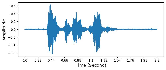
1. Audio Preprocessing
Trimming
- 60dB 이하를 무음으로 처리합니다.
top_dbㅣ 음성 신호의 최대 소음 레벨을 나타내는 변수로 이 값보다 작은 레벨의 소음은 삭제됩니다.frame_lengthㅣ 프레임 길이를 나타내는 변수로, 음성 데이터를 프레임으로 나눌 때 사용됩니다.frame_strideㅣ 프레임 간격을 나타내는 변수로, 연속적인 프레임 사이의 간격을 조절합니다.
1
2
3
4
5
6
7
8
9
10
11
12
13
14
def trimming(data, sampling_rate, top_db = 60):

    frame_length = 0.025   # 0.025 ~ 0.05
    frame_stride = 0.010   # frame_length/2

    input_nfft = int(round(sampling_rate*frame_length))
    input_stride = int(round(sampling_rate*frame_stride))

    if len(np.shape(data)) == 1:
        trim_data = librosa.effects.trim(data, top_db=top_db, frame_length=input_nfft, hop_length=input_stride)[0]
    else:
        trim_data = data.apply(lambda x : librosa.effects.trim(x, top_db=top_db, frame_length=input_nfft, hop_length=input_stride)[0])

    return trim_data
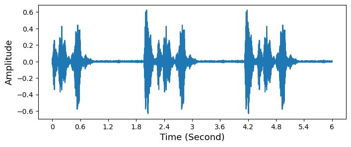
Random Padding
- 음성 데이터들의 길이가 서로 다른 경우 Melspectrogram, MFCC 모두 길이가 다르므로, 고정 사이즈를 정하고 랜덤으로 앞과 뒤에 Padding을 해줍니다.
reqlenㅣ 필요한 최종 데이터 길이- 입력 데이터의 길이가
reqlen보다 길 경우,reqlen에 맞게 데이터를 잘라서 반환합니다. - 입력 데이터의 길이가
reqlen과 같을 경우, 그대로 반환합니다. - 입력 데이터의 길이가
reqlen보다 짧을 경우, 부족한 부분을 랜덤한 값으로 채워서 데이터의 길이를reqlen에 맞게 확장합니다.
- 입력 데이터의 길이가
1
2
3
4
5
6
7
8
9
10
11
12
13
14
15
def padding(x, reqlen=100000):
    x_len = x.shape[0]
    if reqlen < x_len:
        max_offset = x_len - reqlen
        offset = np.random.randint(max_offset)
        x = x[offset:(reqlen+offset)]
        return x
    elif reqlen == x_len:
        return x
    else:
        total_diff = reqlen - x_len
        offset = np.random.randint(total_diff)
        left_pad = offset
        right_pad = total_diff - offset
        return np.pad(x, (left_pad, right_pad), 'wrap')
2. Audio Feature Extraction
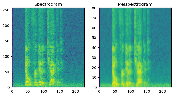
Spectrogram
- Shape ㅣ [주파수 방향 성분 수 (n_fft / 2 + 1,
0Hz부터sample_rate의 절반), Time 방향 성분 수]sample_rate의 절반인 이유 ㅣ Nyquist Frequency
torchaudio,nn.SequentialAmplitudeToDBㅣ Power 단위의 Spectrogram 또는 Melspectrogram을 dB(로그) 단위로 변환합니다.- dB 단위는 딥러닝 모델이 이해하기 편한 범위의 값을 제공합니다.
n_fftㅣwin_length의 크기로 잘린 음성의 작은 조각은 0으로 Padding 되어서n_fft로 크기가 맞춰집니다.- 따라서,
n_fft는win_length보다 크거나 같아야 하고 일반적으로 속도를 위해서2^n의 값으로 설정합니다. - Padding된 조각에 Fourier Transform이 적용되는 것입니다.
- 따라서,
win_lengthㅣ 음성을 잘라서 생기는 작은 조각의 크기입니다.- 16000Hz인 음성에서는
400에 해당하는 값입니다.
- 16000Hz인 음성에서는
hop_lengthㅣ 음성을 작은 조각으로 자를 때 자르는 간격에 해당합니다.- 16000Hz인 음성에서는 160에 해당하는 값
1
2
3
4
5
6
7
8
spectrogram = nn.Sequential(
    AT.Spectrogram(n_fft=512,
                   win_length=400,
                   hop_length=160),
    AT.AmplitudeToDB()
)

spec = spectrogram(sample_data)
Melspectrogram
- 음성데이터를 Frequency, Time의 2차원 도메인으로 변환합니다.
- Shape ㅣ [주파수 방향 성분 수, Time 방향 성분 수]
librosa.feature.melspectrogramn_melsㅣ Melspectrogram의 주파수 해상도를 조절합니다.power_to_dbㅣ Melspectrogram을 데시벨로 스케일링하여 특징을 강조합니다.ref=np.maxㅣ 데시벨로 변환 시 사용되는 참조 값입니다.
1
2
3
4
# Library 1: Librosa
S = librosa.feature.melspectrogram(data, sr=sample_rate, n_mels=40)
log_S = librosa.power_to_db(S, ref=np.max)
librosa.display.specshow(log_S, sr=sr)  # x axis: Time, y axis: Frequency
torchaudio,nn.Sequentialn_melsㅣ 적용할 Mel Filter의 개수를 의미합니다.
1
2
3
4
5
6
7
8
9
10
# Library 2: Torchaudio
mel_spectrogram = nn.Sequential(
    AT.MelSpectrogram(sample_rate=22,
                      n_fft=512,
                      win_length=400,
                      hop_length=160,
                      n_mels=80),
    AT.AmplitudeToDB()
)
mel = mel_spectrogram(sample_data)
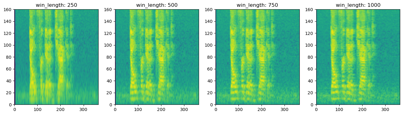
win_length가 커질수록 주파수 성분에 대한 해상도는 높아지지만, 시간 성분에 대한 해상도는 낮아집니다.win_length가 작은 경우에는 주파수 성분에 대한 해상도는 낮아지지만, 시간 성분에 대한 해상도는 높아지게 됩니다.n_fft를 높이면 주파수 성분의 수는 증가하지만 실제 주파수의 해상도는 증가하지 않습니다.
MFCC
1
2
mfcc = librosa.feature.mfcc(data, sr=sample_rate, n_mels=40)
librosa.display.specshow(mfcc, sr=sample_rate)  # x axis: Time, y axis: MFCC coefficients
Stacked Melspectrogram
- Melspectrogram의 1차 미분과 2차 미분을 채널로 Stacking 하여 음성에 대한 변화율 정보를 포함하는 데이터를 생성합니다.
1
2
3
4
5
6
7
8
9
10
11
12
13
14
15
16
17
18
19
20
21
22
23
24
25
26
27
28
29
30
31
32
33
34
35
36
def stacked_melspectrogram(data):

    frame_length = 0.025
    frame_stride = 0.010

    input_nfft = int(round(sampling_rate*frame_length))
    input_stride = int(round(sampling_rate*frame_stride))

    extracted_features = []
    for i in data:

        if feature == "mfcc":
            n_feature = 40
            S = librosa.feature.mfcc(y=i,
                                     sr=sampling_rate,
                                     n_mfcc=n_feature,
                                     n_fft=input_nfft,
                                     hop_length=input_stride)
            S_delta = librosa.feature.delta(S)
            S_delta2 = librosa.feature.delta(S, order=2)

        elif feature == "melspec":
            n_feature = 128
            S = librosa.feature.melspectrogram(y=i,
                                               sr=sampling_rate,
                                               n_mels=n_feature,
                                               n_fft=input_nfft,
                                               hop_length=input_stride)
            S = librosa.power_to_db(S, ref=np.max)
            S_delta = librosa.feature.delta(S)
            S_delta2 = librosa.feature.delta(S, order=2)

        S = np.stack((S, S_delta, S_delta2), axis=2)
        extracted_features.append(S)

    return np.array(extracted_features)
Multi-Resolution Melspectrogram
- 4가지의 서로 다른
win_length로 다양한 해상도를 가진 Melspectrogram들을 Stacking하고 Normalizing 합니다.
1
2
3
4
5
6
7
8
9
10
11
12
13
14
15
16
17
def melspectrogram(win_length):
        mels = nn.Sequential(
            AT.MelSpectrogram(sample_rate=16000, n_fft=2048, win_length=win_length,
                              hop_length=100, pad=50,f_min=25,f_max=7500,n_mels=160),
            AT.AmplitudeToDB())
        return mels

mels_1 = melspectrogram(250)[0, :, 1:-1]
mels_2 = melspectrogram(500)[0, :, 1:-1]
mels_3 = melspectrogram(750)[0, :, 1:-1]
mels_4 = melspectrogram(1000)[0, :, 1:-1]

device = 'cuda' if torch.cuda.is_available() else 'cpu'
cali = torch.linspace(-0.5, 0.5, steps=160, device=device).view(1, -1, 1)

stacked_mels = torch.stack([mels_1, mels_2, mels_3, mels_4], dim=0)
stacked_mels = (stacked_mels - stacked_mels.mean(dim=[1, 2], keepdim=True)) / 20 + cali
3. Data Augmentation
Noising
- 랜덤 노이즈를 추가합니다.
1
2
3
4
5
def noising(data,noise_factor):
    noise = np.random.randn(len(data))
    augmented_data = data + noise_factor * noise
    augmented_data = augmented_data.astype(type(data[0]))
    return augmented_data
Shifting
- 좌우로 이동시킵니다.
1
2
3
4
5
6
7
8
9
10
11
12
13
14
15
def shifting(data, sampling_rate, shift_max, shift_direction):
    shift = np.random.randint(sampling_rate * shift_max+1)
    if shift_direction == 'right':
        shift = -shift
    elif shift_direction == 'both':
        direction = np.random.randint(0, 2)
        if direction == 1:
            shift = -shift
    augmented_data = np.roll(data, shift)
    # Set to silence for heading/ tailing
    if shift > 0:
        augmented_data[:shift] = 0
    else:
        augmented_data[shift:] = 0
    return augmented_data
Pitch
- 피치를 조절합니다.
1
2
def change_pitch(data, sampling_rate, pitch_factor):
    return librosa.effects.pitch_shift(data, sampling_rate, pitch_factor)
SpecAugment
feat_size및seq_len을 계산하여 Spectrogram의 크기를 가져옵니다.freq_mask를 적용하여 주어진freq_mask_num만큼 주파수 축에서 일부 주파수를 무작위로 제거하여 데이터를 변형합니다.time_mask를 적용하여 주어진time_mask_num만큼 시간 축에서 일부 시간적인 정보를 무작위로 제거하여 데이터를 변형합니다.
1
2
3
4
5
6
7
8
9
10
11
12
13
14
15
16
17
18
19
20
21
22
time_mask = 32
freq_mask = 32
n_time_mask = 1
n_freq_mask = 1

def SpecAugment(spec, T=time_mask, F=freq_mask, time_mask_num=n_time_mask, freq_mask_num=n_freq_mask):
    feat_size = spec.shape[0]
    seq_len = spec.shape[1]

    # freq mask
    for _ in range(freq_mask_num):
        f = np.random.uniform(low=0.0, high=F)
        f = int(f)
        f0 = random.randint(0, feat_size - f)
        spec[:, f0 : f0 + f] = 0
    # time mask
    for _ in range(time_mask_num):
        t = np.random.uniform(low=0.0, high=T)
        t = int(t)
        t0 = random.randint(0, seq_len - t)
        spec[t0 : t0 + t] = 0
    return spec
이러한 기법들을 비교하면서 모델에 맞는 특성을 선택하여 사용한다면 AI 예측 성능을 향상시킬 수 있습니다.
This post is licensed under CC BY 4.0 by the author.