인구 데이터 기반 소득 예측하기 | 데이콘
👨👧👧 인구 데이터를 EDA하고 LightGBM과 XGBoost 모델을 활용하여 인구 별 소득을 예측하는 방법을 공유합니다.

인구 데이터 기반 소득 예측하기 | 데이콘
KEYWORDS
소득 예측 머신러닝, 소득 예측 딥러닝, 소득 예측 파이썬, Forecasting Income, LightGBM, XGBoost, Ensemble
데이콘의 “인구 데이터 기반 소득 예측 경진대회”에 참여하여 작성한 글이며, 코드실행은 Google Colab의 GPU, Standard RAM 환경에서 진행했습니다.
➔ 데이콘에서 읽기
0. Import Packages
- 라이브러리 불러오기
1
2
3
4
5
6
7
8
9
10
11
12
13
14
15
16
17
18
19
20
21
22
23
24
25
26
!pip install -U pandas-profiling
import numpy as np
import pandas as pd
import matplotlib
import matplotlib.pyplot as plt
import sklearn
import pandas_profiling
import seaborn as sns
import random as rn
import os
import scipy.stats as stats

from sklearn.preprocessing import LabelEncoder
from sklearn.preprocessing import OneHotEncoder
from sklearn.model_selection import train_test_split
from sklearn.ensemble import VotingClassifier
from sklearn import metrics

import xgboost as xgb
import lightgbm as lgb

from collections import Counter
import warnings

%matplotlib inline
warnings.filterwarnings(action='ignore')
- 주요 라이브러리 버전 확인
1
2
3
4
5
6
print("numpy version: {}". format(np.__version__))
print("pandas version: {}". format(pd.__version__))
print("matplotlib version: {}". format(matplotlib.__version__))
print("scikit-learn version: {}". format(sklearn.__version__))
print("xgboost version: {}". format(xgb.__version__))
print("lightgbm version: {}". format(lgb.__version__))
    numpy version: 1.21.6
    pandas version: 1.3.5
    matplotlib version: 3.2.2
    scikit-learn version: 1.0.2
    xgboost version: 0.90
    lightgbm version: 2.2.3
- 랜덤 시드 고정
1
2
3
4
5
# reproducibility
seed_num = 42
np.random.seed(seed_num)
rn.seed(seed_num)
os.environ['PYTHONHASHSEED']=str(seed_num)
1. Load and Check Dataset
Variable Description
| age | workclass | fnlwgt | education |
| 나이 | 일 유형 | CPS(Current Population Survey) 가중치 | 교육수준 |
| education.num | marital.status | occupation |
| 교육수준 번호 | 결혼 상태 | 직업 |
| relationship | race | sex | capital.gain | capital.loss | hours.per.week | native.country |
| 가족관계 | 인종 | 성별 | 자본 이익 | 자본 손실 | 주당 근무시간 | 본 국적 |
- 데이터 불러오기
1
2
3
4
5
6
7
train = pd.read_csv('/content/drive/MyDrive/Forecasting_income/dataset/train.csv')
test = pd.read_csv('/content/drive/MyDrive/Forecasting_income/dataset/test.csv')

train.columns = train.columns.str.replace('.','_')
test.columns = test.columns.str.replace('.','_')

train.head()
       id  age workclass  fnlwgt     education  education_num      marital_status  \
    0   0   32   Private  309513    Assoc-acdm             12  Married-civ-spouse
    1   1   33   Private  205469  Some-college             10  Married-civ-spouse
    2   2   46   Private  149949  Some-college             10  Married-civ-spouse
    3   3   23   Private  193090     Bachelors             13       Never-married
    4   4   55   Private   60193       HS-grad              9            Divorced

            occupation   relationship   race     sex  capital_gain  capital_loss  \
    0     Craft-repair        Husband  White    Male             0             0
    1  Exec-managerial        Husband  White    Male             0             0
    2     Craft-repair        Husband  White    Male             0             0
    3     Adm-clerical      Own-child  White  Female             0             0
    4     Adm-clerical  Not-in-family  White  Female             0             0

       hours_per_week native_country  target
    0              40  United-States       0
    1              40  United-States       1
    2              40  United-States       0
    3              30  United-States       0
    4              40  United-States       0
- Pandas Profiling Report 생성하기
1
2
pr=train.profile_report()
pr.to_file('/content/drive/MyDrive/Forecasting_income/pr_report.html')
- Pandas Profiling을 활용하면 아래와 같이 데이터 프레임을 쉽고 효율적으로 탐색할 수 있습니다.

Pandas Profiling Report의 Alert 활용하기
Variable Pairs with the High Correlation
relationship-sexage-marital.statusworkclass-occupationeducation-education.numrelationship-marital.statusrace-native.countrysex-occupationtarget-relationship
Data Type
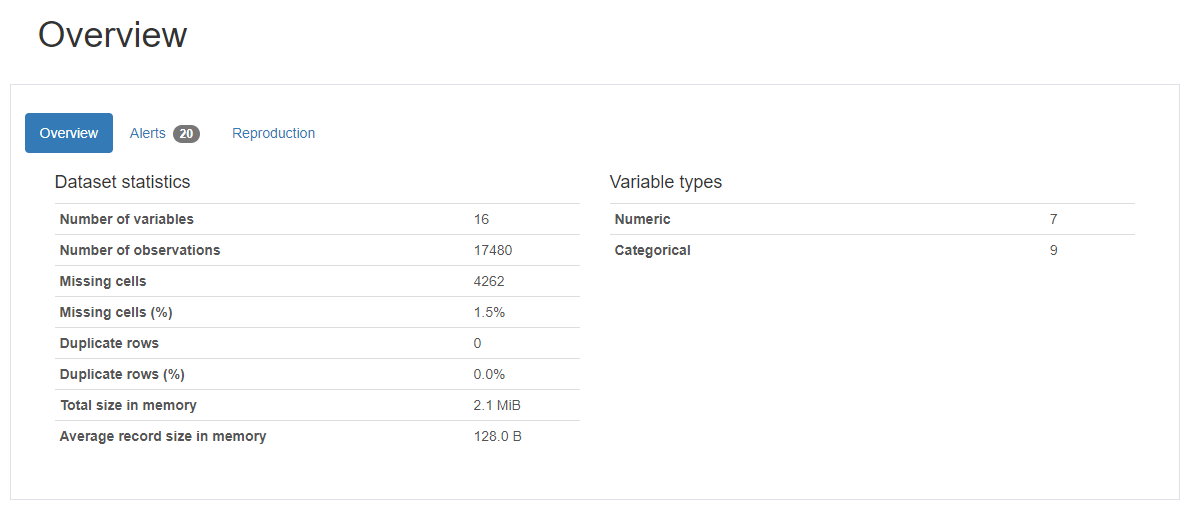
- Numeric (7) :
id,age,fnlwgt,education.num,capital.gain,capital.loss,hours.per.week - Categorical (9) :
workclass,education,marital.status,occupation,relationship,race,sex,native.country,target
Note
workclass와occupation이 같은 비율 (10.5%)의 결측치(Missing Value)를 가집니다.native.country는 583(3.3%)의 결측치(Missing Value)를 가지므로 해당 행(Row)을 삭제해주겠습니다.capital.gain와capital.loss는 높은 왜도(Skewness)를 가집니다. 이상치(Outlier)를 확인하고 필요시 제거하거나 변환 함수를 적용하겠습니다.
1
train.info()
    <class 'pandas.core.frame.DataFrame'>
    RangeIndex: 17480 entries, 0 to 17479
    Data columns (total 16 columns):
     #   Column          Non-Null Count  Dtype
    ---  ------          --------------  -----
     0   id              17480 non-null  int64
     1   age             17480 non-null  int64
     2   workclass       15644 non-null  object
     3   fnlwgt          17480 non-null  int64
     4   education       17480 non-null  object
     5   education_num   17480 non-null  int64
     6   marital_status  17480 non-null  object
     7   occupation      15637 non-null  object
     8   relationship    17480 non-null  object
     9   race            17480 non-null  object
     10  sex             17480 non-null  object
     11  capital_gain    17480 non-null  int64
     12  capital_loss    17480 non-null  int64
     13  hours_per_week  17480 non-null  int64
     14  native_country  16897 non-null  object
     15  target          17480 non-null  int64
    dtypes: int64(8), object(8)
    memory usage: 2.1+ MB
2. Data Preprocessing
(1) Missing Value
1
train.columns[train.isnull().any()]
Index(['workclass', 'occupation', 'native_country'], dtype='object')
1
train[train["workclass"].isnull()]
              id  age workclass  fnlwgt     education  education_num  \
    15081  15081   90       NaN   77053       HS-grad              9
    15082  15082   66       NaN  186061  Some-college             10
    15084  15084   51       NaN  172175     Doctorate             16
    15086  15086   61       NaN  135285       HS-grad              9
    15087  15087   71       NaN  100820       HS-grad              9
    ...      ...  ...       ...     ...           ...            ...
    17475  17475   35       NaN  320084     Bachelors             13
    17476  17476   30       NaN   33811     Bachelors             13
    17477  17477   71       NaN  287372     Doctorate             16
    17478  17478   41       NaN  202822       HS-grad              9
    17479  17479   72       NaN  129912       HS-grad              9

               marital_status occupation   relationship                race  \
    15081             Widowed        NaN  Not-in-family               White
    15082             Widowed        NaN      Unmarried               Black
    15084       Never-married        NaN  Not-in-family               White
    15086  Married-civ-spouse        NaN        Husband               White
    15087  Married-civ-spouse        NaN        Husband               White
    ...                   ...        ...            ...                 ...
    17475  Married-civ-spouse        NaN           Wife               White
    17476       Never-married        NaN  Not-in-family  Asian-Pac-Islander
    17477  Married-civ-spouse        NaN        Husband               White
    17478           Separated        NaN  Not-in-family               Black
    17479  Married-civ-spouse        NaN        Husband               White

              sex  capital_gain  capital_loss  hours_per_week native_country  \
    15081  Female             0          4356              40  United-States
    15082  Female             0          4356              40  United-States
    15084    Male             0          2824              40  United-States
    15086    Male             0          2603              32  United-States
    15087    Male             0          2489              15  United-States
    ...       ...           ...           ...             ...            ...
    17475  Female             0             0              55  United-States
    17476  Female             0             0              99  United-States
    17477    Male             0             0              10  United-States
    17478  Female             0             0              32  United-States
    17479    Male             0             0              25  United-States

           target
    15081       0
    15082       0
    15084       1
    15086       0
    15087       0
    ...       ...
    17475       1
    17476       0
    17477       1
    17478       0
    17479       0

    [1836 rows x 16 columns]
1
train['workclass'].unique()
    array(['Private', 'State-gov', 'Local-gov', 'Self-emp-not-inc',
           'Self-emp-inc', 'Federal-gov', 'Without-pay', nan, 'Never-worked'],
          dtype=object)
workclass와occupation열(Column)에서 결측치가 포함된 행은 삭제합니다.- 두 열이 동시에 결측치를 갖는 경우가 대부분이므로,
workclass의 결측치만Never-worked와 같은 이미 존재하는 특성으로 채우는 것은 의미가 없습니다. workclass와occupation에 새로운 feature을 부여하는 방법도 시도하였지만, One-hot Encoding을 했을 때 생기는 테스트 데이터와의 값 차이 때문에 다른 방법을 고려해볼 필요가 있다고 생각합니다 😔
1
2
3
4
print(sum(train['workclass'].isna()))
print(sum(train['occupation'].isna()))

fill_na = train['workclass'].isna()
    1836
    1843
1
2
3
4
5
df_train = train.dropna()

print(sum(df_train['workclass'].isna()))
print(sum(df_train['occupation'].isna()))
print(sum(df_train['native_country'].isna()))
    0
    0
    0
1
df_train
              id  age     workclass  fnlwgt     education  education_num  \
    0          0   32       Private  309513    Assoc-acdm             12
    1          1   33       Private  205469  Some-college             10
    2          2   46       Private  149949  Some-college             10
    3          3   23       Private  193090     Bachelors             13
    4          4   55       Private   60193       HS-grad              9
    ...      ...  ...           ...     ...           ...            ...
    15076  15076   35       Private  337286       Masters             14
    15077  15077   36       Private  182074  Some-college             10
    15078  15078   50  Self-emp-inc  175070   Prof-school             15
    15079  15079   39       Private  202937  Some-college             10
    15080  15080   33       Private   96245    Assoc-acdm             12

               marital_status       occupation   relationship                race  \
    0      Married-civ-spouse     Craft-repair        Husband               White
    1      Married-civ-spouse  Exec-managerial        Husband               White
    2      Married-civ-spouse     Craft-repair        Husband               White
    3           Never-married     Adm-clerical      Own-child               White
    4                Divorced     Adm-clerical  Not-in-family               White
    ...                   ...              ...            ...                 ...
    15076       Never-married  Exec-managerial  Not-in-family  Asian-Pac-Islander
    15077            Divorced     Adm-clerical  Not-in-family               White
    15078  Married-civ-spouse   Prof-specialty        Husband               White
    15079            Divorced     Tech-support  Not-in-family               White
    15080  Married-civ-spouse   Prof-specialty        Husband               White

              sex  capital_gain  capital_loss  hours_per_week native_country  \
    0        Male             0             0              40  United-States
    1        Male             0             0              40  United-States
    2        Male             0             0              40  United-States
    3      Female             0             0              30  United-States
    4      Female             0             0              40  United-States
    ...       ...           ...           ...             ...            ...
    15076    Male             0             0              40  United-States
    15077    Male             0             0              45  United-States
    15078    Male             0             0              45  United-States
    15079  Female             0             0              40         Poland
    15080    Male             0             0              50  United-States

           target
    0           0
    1           1
    2           0
    3           0
    4           0
    ...       ...
    15076       0
    15077       0
    15078       1
    15079       0
    15080       0

    [15081 rows x 16 columns]
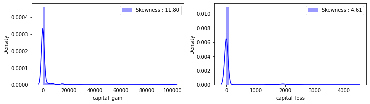
(2) Outlier
1
2
3
4
5
6
7
fig, ax = plt.subplots(1, 2, figsize=(12,3))
g = sns.distplot(df_train['capital_gain'], color='b', label='Skewness : {:.2f}'.format(df_train['capital_gain'].skew()), ax=ax[0])
g = g.legend(loc='best')

g = sns.distplot(df_train['capital_loss'], color='b', label='Skewness : {:.2f}'.format(df_train['capital_loss'].skew()), ax=ax[1])
g = g.legend(loc='best')
plt.show()
1
2
3
4
5
6
7
8
9
10
11
12
13
14
15
16
numeric_fts = ['age', 'fnlwgt', 'education_num', 'capital_gain', 'capital_loss', 'hours_per_week']

outlier_ind = []
for i in numeric_fts:
  Q1 = np.percentile(df_train[i],25)
  Q3 = np.percentile(df_train[i],75)
  IQR = Q3-Q1
  outlier_list = df_train[(df_train[i] < Q1 - IQR * 1.5) | (df_train[i] > Q3 + IQR * 1.5)].index
  outlier_ind.extend(outlier_list)

outlier_ind = Counter(outlier_ind)
multi_outliers = list(k for k,j in outlier_ind.items() if j > 2)

# Drop outliers
train_df = df_train.drop(multi_outliers, axis = 0).reset_index(drop = True)
train_df
              id  age     workclass  fnlwgt     education  education_num  \
    0          0   32       Private  309513    Assoc-acdm             12
    1          1   33       Private  205469  Some-college             10
    2          2   46       Private  149949  Some-college             10
    3          3   23       Private  193090     Bachelors             13
    4          4   55       Private   60193       HS-grad              9
    ...      ...  ...           ...     ...           ...            ...
    15043  15076   35       Private  337286       Masters             14
    15044  15077   36       Private  182074  Some-college             10
    15045  15078   50  Self-emp-inc  175070   Prof-school             15
    15046  15079   39       Private  202937  Some-college             10
    15047  15080   33       Private   96245    Assoc-acdm             12

               marital_status       occupation   relationship                race  \
    0      Married-civ-spouse     Craft-repair        Husband               White
    1      Married-civ-spouse  Exec-managerial        Husband               White
    2      Married-civ-spouse     Craft-repair        Husband               White
    3           Never-married     Adm-clerical      Own-child               White
    4                Divorced     Adm-clerical  Not-in-family               White
    ...                   ...              ...            ...                 ...
    15043       Never-married  Exec-managerial  Not-in-family  Asian-Pac-Islander
    15044            Divorced     Adm-clerical  Not-in-family               White
    15045  Married-civ-spouse   Prof-specialty        Husband               White
    15046            Divorced     Tech-support  Not-in-family               White
    15047  Married-civ-spouse   Prof-specialty        Husband               White

              sex  capital_gain  capital_loss  hours_per_week native_country  \
    0        Male             0             0              40  United-States
    1        Male             0             0              40  United-States
    2        Male             0             0              40  United-States
    3      Female             0             0              30  United-States
    4      Female             0             0              40  United-States
    ...       ...           ...           ...             ...            ...
    15043    Male             0             0              40  United-States
    15044    Male             0             0              45  United-States
    15045    Male             0             0              45  United-States
    15046  Female             0             0              40         Poland
    15047    Male             0             0              50  United-States

           target
    0           0
    1           1
    2           0
    3           0
    4           0
    ...       ...
    15043       0
    15044       0
    15045       1
    15046       0
    15047       0

    [15048 rows x 16 columns]
1
print(train_df['capital_gain'].skew(), train_df['capital_loss'].skew())
12.004940559585881 4.607122286739042
- 이상치들을 제거하였음에도 두 변수는 여전히 높은 왜도를 보이고 있어, 로그 변환(Log Transformation)을 진행했습니다.
1
2
3
4
5
6
7
8
# log transformation
train_df['capital_gain'] = train_df['capital_gain'].map(lambda i: np.log(i) if i > 0 else 0)
test['capital_gain'] = test['capital_gain'].map(lambda i: np.log(i) if i > 0 else 0)

train_df['capital_loss'] = train_df['capital_loss'].map(lambda i: np.log(i) if i > 0 else 0)
test['capital_loss'] = test['capital_loss'].map(lambda i: np.log(i) if i > 0 else 0)

print(train_df['capital_gain'].skew(), train_df['capital_loss'].skew())
3.0945787119106676 4.390015583095806
3. Feature Engineering
(1) Correlation
- 범주형(Categorical) 데이터를 라벨 인코더(Label Encoder)를 통해 수치형(Numerical)으로 변환한 후 상관관계를 확인합니다.
- Categorical :
workclass,education,marital.status,occupation,relationship,race,sex,native.country
1
2
3
4
5
6
7
8
la_train = train_df.copy()

cat_fts = ['workclass', 'education', 'marital_status', 'occupation', 'relationship', 'race', 'sex', 'native_country']
for i in range(len(cat_fts)):
  encoder = LabelEncoder()
  la_train[cat_fts[i]] = encoder.fit_transform(la_train[cat_fts[i]])

la_train.head()
       id  age  workclass  fnlwgt  education  education_num  marital_status  \
    0   0   32          2  309513          7             12               2
    1   1   33          2  205469         15             10               2
    2   2   46          2  149949         15             10               2
    3   3   23          2  193090          9             13               4
    4   4   55          2   60193         11              9               0

       occupation  relationship  race  sex  capital_gain  capital_loss  \
    0           2             0     4    1           0.0           0.0
    1           3             0     4    1           0.0           0.0
    2           2             0     4    1           0.0           0.0
    3           0             3     4    0           0.0           0.0
    4           0             1     4    0           0.0           0.0

       hours_per_week  native_country  target
    0              40              38       0
    1              40              38       1
    2              40              38       0
    3              30              38       0
    4              40              38       0
- 앞서 수행한 Pandas Profiling Report의 Alert 섹션을 참고하여 상관계수를 계산했습니다.
- 유의미한 상관관계를 가지고 있다고 생각되는 변수 Pair는
relationship-sex,occupation-workclass,education-education.num입니다.
1
2
# Pearson
la_train[['age','marital_status', 'relationship', 'sex', 'occupation', 'workclass']].corr()
                         age  marital_status  relationship       sex  occupation  \
    age             1.000000       -0.271955     -0.240331  0.087515   -0.007994
    marital_status -0.271955        1.000000      0.180281 -0.124481    0.023856
    relationship   -0.240331        0.180281      1.000000 -0.590077   -0.052109
    sex             0.087515       -0.124481     -0.590077  1.000000    0.061443
    occupation     -0.007994        0.023856     -0.052109  0.061443    1.000000
    workclass       0.081100       -0.044000     -0.070512  0.078764    0.010194

                    workclass
    age              0.081100
    marital_status  -0.044000
    relationship    -0.070512
    sex              0.078764
    occupation       0.010194
    workclass        1.000000
1
la_train[['education', 'education_num', 'race', 'native_country']].corr()
                    education  education_num      race  native_country
    education        1.000000       0.348614  0.011236        0.079063
    education_num    0.348614       1.000000  0.034686        0.097485
    race             0.011236       0.034686  1.000000        0.126654
    native_country   0.079063       0.097485  0.126654        1.000000
범주형인 변수는 Cramer’s V 공식을 활용하여 상관관계를 확인했습니다.
\(V = \sqrt{\frac{\chi^2}{N \cdot \min(k-1, r-1)}}\)
- $N$: 전체 관측값의 합
- $k$: 행의 개수
- $r$: 열의 개수
1
2
3
4
5
6
7
stat = stats.chi2_contingency(la_train[['race', 'native_country']].values, correction=False)[0]
obs = np.sum(la_train[['race', 'native_country']].values)
mini = min(la_train[['race', 'native_country']].values.shape)-1

# Cramer's V
V = np.sqrt((stat/(obs*mini)))
print(V)
0.11306993147326666
(2) String to numerical
- 범주형 데이터를 모델의 Input으로 사용하기 위해서는 수치형 데이터로 변환시킬 필요가 있습니다. 라벨 인코더는 불필요한 상관관계를 보일 가능성이 있기에 원핫 인코더(One-hot Encoder)를 사용했습니다.
- Categorical :
workclass,education,marital.status,occupation,relationship,race,sex,native.country
1
2
train_dataset = train_df.copy()
test_dataset = test.copy()
get_dummies를 사용하여 원핫 인코딩을 진행했습니다.
1
2
3
4
5
train_dataset = pd.get_dummies(train_dataset)
test_dataset = pd.get_dummies(test_dataset)

print(train_dataset.columns)
print(test_dataset.columns)
    Index(['id', 'age', 'fnlwgt', 'education_num', 'capital_gain', 'capital_loss',
           'hours_per_week', 'target', 'workclass_Federal-gov',
           'workclass_Local-gov',
           ...
           'native_country_Portugal', 'native_country_Puerto-Rico',
           'native_country_Scotland', 'native_country_South',
           'native_country_Taiwan', 'native_country_Thailand',
           'native_country_Trinadad&Tobago', 'native_country_United-States',
           'native_country_Vietnam', 'native_country_Yugoslavia'],
          dtype='object', length=106)
    Index(['id', 'age', 'fnlwgt', 'education_num', 'capital_gain', 'capital_loss',
           'hours_per_week', 'workclass_Federal-gov', 'workclass_Local-gov',
           'workclass_Private',
           ...
           'native_country_Portugal', 'native_country_Puerto-Rico',
           'native_country_Scotland', 'native_country_South',
           'native_country_Taiwan', 'native_country_Thailand',
           'native_country_Trinadad&Tobago', 'native_country_United-States',
           'native_country_Vietnam', 'native_country_Yugoslavia'],
          dtype='object', length=104)
- Train 데이터와 Test 데이터의 열 길이를 맞춰주는 작업을 합니다.
1
2
3
4
5
6
7
8
9
test_col = []
add_test = []

for i in test_dataset.columns:
    test_col.append(i)
for j in train_dataset.columns:
    if j not in test_col:
        add_test.append(j)
add_test.remove('target')
- Test 데이터의
native.country열에는 ‘Holand-Netherlands’ 특성이 없는걸까요?
1
print(add_test)
['native_country_Holand-Netherlands']
1
2
3
4
5
for d in add_test:
    test_dataset[d] = 0

print(train_dataset.columns)
print(test_dataset.columns)
    Index(['id', 'age', 'fnlwgt', 'education_num', 'capital_gain', 'capital_loss',
           'hours_per_week', 'target', 'workclass_Federal-gov',
           'workclass_Local-gov',
           ...
           'native_country_Portugal', 'native_country_Puerto-Rico',
           'native_country_Scotland', 'native_country_South',
           'native_country_Taiwan', 'native_country_Thailand',
           'native_country_Trinadad&Tobago', 'native_country_United-States',
           'native_country_Vietnam', 'native_country_Yugoslavia'],
          dtype='object', length=106)
    Index(['id', 'age', 'fnlwgt', 'education_num', 'capital_gain', 'capital_loss',
           'hours_per_week', 'workclass_Federal-gov', 'workclass_Local-gov',
           'workclass_Private',
           ...
           'native_country_Puerto-Rico', 'native_country_Scotland',
           'native_country_South', 'native_country_Taiwan',
           'native_country_Thailand', 'native_country_Trinadad&Tobago',
           'native_country_United-States', 'native_country_Vietnam',
           'native_country_Yugoslavia', 'native_country_Holand-Netherlands'],
          dtype='object', length=105)
- Train 데이터의 Target 열을 제외하면, 열 길이가 잘 맞춰진것을 확인할 수 있습니다.
4. Modeling
- 먼저, Train과 Validation 데이터를
train_test_split함수를 사용하여 만들어줍니다.
1
2
3
4
5
6
7
8
9
10
11
12
13
14
test_size =0.15

train_data, val_data = train_test_split(train_dataset, test_size = test_size, random_state = seed_num)

drop_col = ['target', 'id']

train_x = train_data.drop(drop_col, axis = 1)
train_y = pd.DataFrame(train_data['target'])

val_x = val_data.drop(drop_col, axis = 1)
val_y = pd.DataFrame(val_data['target'])

print(train_x.shape, train_y.shape)
print(val_x.shape, val_y.shape)
    (12790, 104) (12790, 1)
    (2258, 104) (2258, 1)
- LGBM과 XGboost를 Soft Voting하여 간단한 앙상블(Ensemble) 파이프라인을 제작했습니다.
- Soft Voting은 LGBM, XGboost 모델의 예측 확률을 평균 계산하여 최종 Class를 결정합니다.
1
2
3
4
5
6
7
8
9
10
11
12
13
14
15
16
LGBClassifier = lgb.LGBMClassifier(random_state = seed_num)
lgbm = LGBClassifier.fit(train_x.values,
                       train_y.values.ravel(),
                       eval_set = [(train_x.values, train_y), (val_x.values, val_y)],
                       eval_metric ='auc', early_stopping_rounds = 1000,
                       verbose = True)

XGBClassifier = xgb.XGBClassifier(max_depth = 6, learning_rate = 0.01, n_estimators = 10000, random_state = seed_num)
xgb = XGBClassifier.fit(train_x.values,
                       train_y.values.ravel(),
                       eval_set = [(train_x.values, train_y), (val_x.values, val_y)],
                       eval_metric = 'auc', early_stopping_rounds = 1000,
                       verbose = True)

voting = VotingClassifier(estimators=[('xgb', xgb),('lgbm', lgbm)], voting='soft')
vot = voting.fit(train_x.values, train_y.values)
5. Evaluation & Submission
1
2
3
4
5
6
7
l_val_y_pred = lgbm.predict(val_x.values)
x_val_y_pred = xgb.predict(val_x.values)
v_val_y_pred = vot.predict(val_x.values)

print(metrics.accuracy_score(l_val_y_pred, val_y))
print(metrics.accuracy_score(x_val_y_pred, val_y))
print(metrics.accuracy_score(v_val_y_pred, val_y))
    0.8702391496899912
    0.8680248007085917
    0.8596102745792737
1
print(metrics.classification_report(v_val_y_pred, val_y))
                  precision    recall  f1-score   support

               0       0.93      0.89      0.91      1800
               1       0.63      0.72      0.68       458

        accuracy                           0.86      2258
       macro avg       0.78      0.81      0.79      2258
    weighted avg       0.87      0.86      0.86      2258
1
2
3
4
5
6
val_xgb = pd.Series(l_val_y_pred, name="XGB")
val_lgbm = pd.Series(x_val_y_pred, name="LGBM")

ensemble_results = pd.concat([val_xgb,val_lgbm],axis=1)
sns.heatmap(ensemble_results.corr(), annot=True)
plt.show()

- Soft Voting을 진행했음에도 성능이 향상되지 않았습니다.
- 두 모델의 예측은 높은 상관관계를 가지기 때문에, 앙상블을 해도 성능이 향상되지 않는 것이라 예상해봅니다.
This post is licensed under CC BY 4.0 by the author.